Shantanu Pandey
Projects
Hard Light Vector
Memory Manager
Samurai Crusader
Dyslexia VR
Geriatric Depression Suite
Prototypes
Game Mechanics
Diana's Inferno
MakeUp & BreakUp
10Pest
Ninja Pinball
Blogs
Sic Parvis Magna
Game Engineering - Week 1
Game Engineering - Week 2
Game Engineering - Week 3
Game Engineering - Week 4
Game Engineering - Week 5
Game Engineering - Week 6
Game Engineering - Week 7
Game Engineering - Week 8
Game Engineering - Week 9
Engine Feature - Audio Subsystem
Final Project - GameEngineering III
AI Movement Algorithms
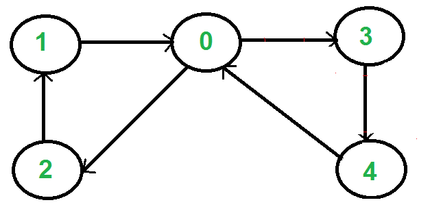
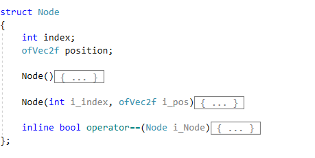
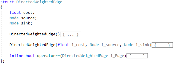
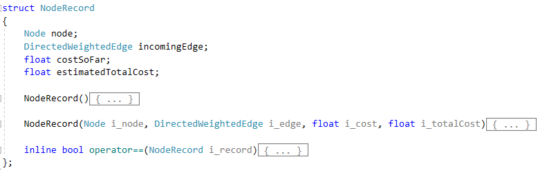
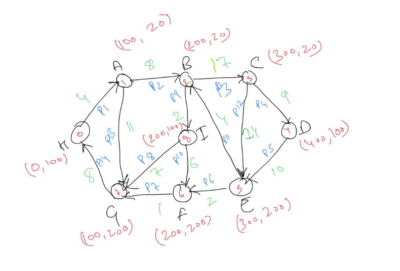
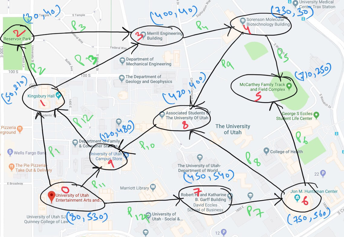
Pathfinding Algortihms
Decision Makiing
About
Projects
Hard Light Vector
Memory Manager
Samurai Crusader
Dyslexia VR
Geriatric Depression Suite
Prototypes
Game Mechanics
Diana's Inferno
MakeUp & BreakUp
10Pest
Ninja Pinball
Blogs
Sic Parvis Magna
Game Engineering - Week 1
Game Engineering - Week 2
Game Engineering - Week 3
Game Engineering - Week 4
Game Engineering - Week 5
Game Engineering - Week 6
Game Engineering - Week 7
Game Engineering - Week 8
Game Engineering - Week 9
Engine Feature - Audio Subsystem
Final Project - GameEngineering III
AI Movement Algorithms
Pathfinding Algortihms
Decision Makiing
About
 RSS Feed